|
|
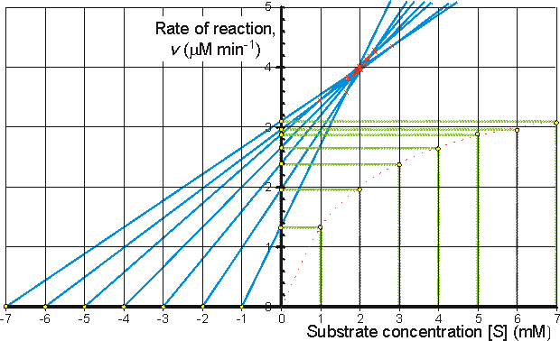
Determination of Vmax and KmIt is important to have as thorough knowledge as is possible of the performance characteristics of enzymes, if they are to be used most efficiently. The kinetic parameters Vmax, Km and kcat/Km should, therefore, be determined. There are two approaches to this problem using either the reaction progress curve (integral method) or the initial rates of reaction (differential method). Use of either method depends on prior knowledge of the mechanism for the reaction and, at least approximately, the optimum conditions for the reaction. If the mechanism is known and complex then the data must be reconciled to the appropriate model (hypothesis), usually by use of a computer-aided analysis involving a weighted least-squares fit. Many such computer programs are currently available and, if not, the programming skill involved is usually fairly low. If the mechanism is not known, initial attempts are usually made to fit the data to the Michaelis-Menten kinetic model. Combining equations (1.1) and (1.8), which, on integration, using the boundary condition that the product is absent at time zero and by substituting [S] by ([S]0 - [P]), becomes If the fractional conversion (X) is introduced, where then equation (1.100) may be simplified to give: Use of equation (1.99) involves the determination of the initial rate of reaction over a wide range of substrate concentrations. The initial rates are used, so that [S] = [S]0, the predetermined and accurately known substrate concentration at the start of the reaction. Its use also ensures that there is no effect of reaction reversibility or product inhibition which may affect the integral method based on equation (1.102). Equation (1.99) can be utilised directly using a computer program, involving a weighted least-squares fit, where the parameters for determining the hyperbolic relationship between the initial rate of reaction and initial substrate concentration (i.e., Km and Vmax) are chosen in order to minimise the errors between the data and the model, and the assumption is made that the errors inherent in the practically determined data are normally distributed about their mean (error-free) value. Alternatively the direct linear plot may be used (Figure 1.10). This is a powerful non-parametric statistical method which depends upon the assumption that any errors in the experimentally derived data are as likely to be positive (i.e., too high) as negative (i.e., too low). It is common practice to show the data obtained by the above statistical methods on one of three linearised plots, derived from equation (1.99) (Figure 1.11). Of these, the double reciprocal plot is preferred to test for the qualitative correctness of a proposed mechanism, and the Eadie-Hofstee plot is preferred for discovering deviations from linearity.
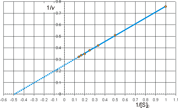
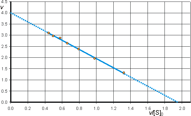
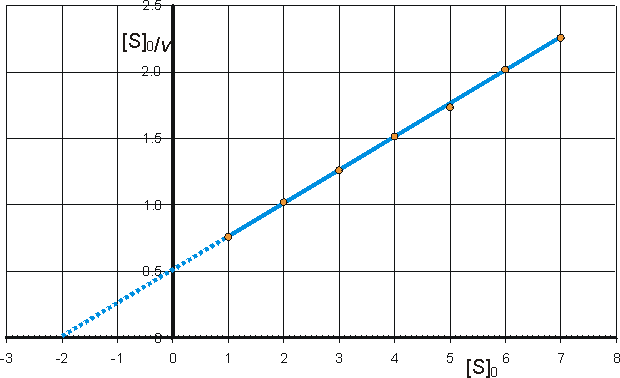
Figure 1.10. The direct linear plot. A plot of the initial rate of reaction against the initial substrate concentration also showing the way estimates can be directly made of the Km and Vmax. Every pair of data points may be utilised to give a separate estimate of these parameters (i.e., n(n-1)/2 estimates from n data points with differing [S]0). These estimates are determined from the intersections of lines passing through the (x,y) points (-[S]0,0) and (0,v); each intersection forming a separate estimate of Km and Vmax. The intersections are separately ranked in order of increasing value of both Km and Vmax and the median values taken as the best estimates for these parameters. The error in these estimates can be simply determined from sub-ranges of these estimates, the width of the sub-range dependent on the accuracy required for the error and the number of data points in the analysis. In this example there are 7 data points and, therefore, 21 estimates for both Km and Vmax. The ranked list of the estimates for Km (mM) is 0.98,1.65, 1.68, 1.70, 1.85, 1.87, 1.89, 1.91, 1.94, 1.96, 1.98, 1.99, 2.03, 2.06, 1.12, 2.16, 2.21, 2.25, 2.38, 2.40, 2.81, with a median value of 1.98 mM. The Km must lie between the 4th (1.70 mM) and 18th (2.25 mM) estimate at a confidence level of 97% (Cornish-Bowden et al., 1978). The list of the estimates for Vmax (mM.min−1) is ranked separately as 3.45, 3.59, 3.80, 3.85, 3.87, 3.89, 3.91, 3.94, 3.96, 3.96, 3.98, 4.01, 4.03, 4.05, 4.13, 4.14, 4.18, 4.26, 4.29, 4.35, with a median value of 3.98 mM.min−1. The Vmax must lie between the 4th (3.85 mM.min−1) and 18th (4.18 mM.min−1) estimate at a confidence level of 97%. It can be seen that outlying estimates have little or no influence on the results. This is a major advantage over the least-squared statistical procedures where rogue data points cause heavily biased effects. Figure 1.11. Three ways in which the hyperbolic relationship between the initial rate of reaction and the initial substrate concentration
can be rearranged to give linear plots. The examples are drawn using Km = 2 mM and Vmax = 4 mM min−1. (a) Lineweaver-Burk (double-reciprocal) plot of 1/v against 1/[S]0 giving intercepts at 1/Vmax and -1/Km
(b) Eadie-Hofstee plot of v against v/[S]0 giving intercepts at Vmax and Vmax/Km
c) Hanes-Woolf (half-reciprocal) plot of [S]0/v against [S]0 giving intercepts at Km/Vmax and Km.
The progress curve of the reaction (Figure 1.12) can be used to determine the specificity constant (kcat/Km) by making use of the relationship between time of reaction and fractional conversion (see equation (1.102). This has the advantage over the use of the initial rates (above) in that fewer determinations need to be made, possibly only one progress curve is necessary, and sometimes the initial rate of reaction is rather difficult to determine due to its rapid decline. If only the early part of the progress curve, or its derivative, is utilised in the analysis, this procedure may even be used in cases where there is competitive inhibition by the product, or where the reaction is reversible.
Figure 1.12. A schematic plot showing the amount of product formed (productivity) against the time of reaction, in a closed system. The specificity constant may be determined by a weighted least-squared fit of the data to the relationship given by equation (1.102). The type of inhibition and the inhibition constants may be determined from the effect of differing concentrations of inhibitor on the apparent Km, Vmax and kcat/Km, although some more specialised plots do exist (e.g., Cornish-Bowden, 1974).
This page was established in 2004 and last updated by Martin
Chaplin |
![t = [P]/Vmax - Km Ln(([S]0 - [P])/( [S]0 ))/Vmax](images/determ18.gif) (1.100)
(1.100)


![{productivity-time curve showing linear increase in product formation with time at the beginning but reaching a maximum product formation after some time]](images/prod.gif)